Three types of materials are defined: fluid materials, solid materials and thermal interface materials (TIM). A material can be assigned to a solid region, fluid region or interface by selecting it from the material list or by defining a new one. The list of materials can be managed through the libraries page. This libraries page contains a list of predefined materials, but you can define your own materials as well. The predefined materials cannot be editted by anyone, your own custom materials can.
All the predefined materials with constant properties are defined at Standard Temperature Pressure (STP) conditions. The STP conditions correspond to a temperature of 273.15 \(K\) or 0 \(° C\) and a pressure of 100 \(kPa\) or 1 \(bar\). The properties for each type of material is given below:
Property
Material type
Name
Unit
Solid
Fluid
TIM
Density \(\rho\)
\(kg/m^{3}\)
Dynamic viscosity \(\mu\)
\(kg/(ms)=Pa*s\)
Specific heat capacity \(C_{p}\)
\(J/(kg \cdot K)\)
Absorption coefficient \(\alpha\)
\(m^{-1}\)
Thermal conductivity \(\kappa\)
\(W/(m \cdot K)\)
Coefficient of thermal expansion \(\beta\)
\(K^{-1}\)
Thickness \(R_{d}\)
\(m\)
Resistivity
\(\Omega*m\)
Thermal resistance \(R_{th}\)
\(K/W\)
Solids
Density \(\rho\)
The density of a material is commonly denoted with the Greek letter rho (\(\rho\)). The density can be set in three ways:
constant value at a reference temperature
polynomial function of temperature where a maximum of 8 coefficients can be provided
table containing temperature and corresponding parameter value of the material at the specified temperature
Specific heat capacity \(C_{p}\)
The specific heat capacity of a material is denoted as \(C_{p}\). According to the thermodynamic models used, \(C_{p}\) can be a constant or a temperature dependent value. In case of a constant, user specified values in \(J/(K \cdot kg)\) are used. Otherwise, \(C_{p}\) as a function of temperature is calculated using the available thermodynamic models. The specific heat capacity can be set in three ways:
constant value at a reference temperature
polynomial function of temperature where a maximum of 8 coefficients can be provided
table containing temperature and corresponding parameter value of the material at the specified temperature
Thermal conductivity \(\kappa\)
The thermal conductivity of a material is denoted with the Greek letter kappa (\(\kappa\)). The thermal conductivity of a material has the unit \(W/(m \cdot K)\). It can be a constant provided by the user or can also be calculated using the transport coefficients from the transport model specified. An anisotropic conductivity can be defined by setting the appropriate thermal conductivity along the x-axis, y-axis, and z-axis. The thermal conductivity can be set in three ways:
constant value at a reference temperature
polynomial function of temperature where a maximum of 8 coefficients can be provided
table containing temperature and corresponding parameter value of the material at the specified temperature
Absorption Coefficient \(\alpha\)
Thermal radiation models can be switched-on for certain types of simulations. For all boundaries, fluid or solid, the emissivity needs to be provided. Solid regions are considered to be participating in radiative heat transfer when radiation is turned on. Therefore, absorption coefficient \(\alpha \) needs to be set for solid regions. Emissivity is a dimensionless number ranging between 0 and 1. Absorption coefficient has unit \(m^{-1}\) and the value depends on the solid material.
Fluids
Density \(\rho\)
The density of a material is commonly denoted with the Greek letter rho (\(\rho\)). The density can be set in three ways:
constant value at a reference temperature
polynomial function of temperature where a maximum of 8 coefficients can be provided
table containing temperature and corresponding parameter value of the material at the specified temperature
Dynamic viscosity \(\mu\)
The dynamic viscosity of a material is commonly denoted with the Greek letter mu (\(\mu\)). It is important to note that we use dynamic viscosity with unit \(Pa \cdot s\) and not the kinematic viscosity. Viscosity should only be defined for fluids. The dynamic viscosity can be set in three ways:
constant value at a reference temperature
polynomial function of temperature where a maximum of 8 coefficients can be provided
table containing temperature and corresponding parameter value of the material at the specified temperature
Specific heat capacity \(C_{p}\)
The specific heat capacity of a material is denoted as \(C_{p}\). According to the thermodynamic models used, \(C_{p}\) can be a constant or a temperature dependent value. In case of a constant, user specified values in \(J/(K \cdot kg)\) are used. Otherwise, \(C_{p}\) as a function of temperature is calculated using the available thermodynamic models. The specific heat capacity can be set in three ways:
constant value at a reference temperature
polynomial function of temperature where a maximum of 8 coefficients can be provided
table containing temperature and corresponding parameter value of the material at the specified temperature
Thermal conductivity \(\kappa\)
The thermal conductivity of a material is denoted with the Greek letter kappa (\(\kappa\)). The thermal conductivity of a material has the unit \(W/(m \cdot K)\). It can be a constant provided by the user or can also be calculated using the transport coefficients from the transport model specified. An anisotropic conductivity can not be defined for fluids. The thermal conductivity can be set in three ways:
constant value at a reference temperature
polynomial function of temperature where a maximum of 8 coefficients can be provided
table containing temperature and corresponding parameter value of the material at the specified temperature
Coefficient of thermal expansion \(\beta\)
Materials change shape, area or volume depending on the change in temperature. Coefficient of thermal expansion denoted as beta (\(\beta\)) is used to quantify this behavior. The unit for thermal expansion coefficient is \(K^{-1}\). The thermal expansion coefficient can be set in three ways:
constant value at a reference temperature
polynomial function of temperature where a maximum of 8 coefficients can be provided
table containing temperature and corresponding parameter value of the material at the specified temperature
Thermal interface materials
The thermal interface is commonly used in thermal management applications to facilitate effective thermal path between components. Examples of thermal interface materials are thermal greases, thermal tapes, etc. Thermal interface materials are defined by two properties - thermal conductivity and the thickness of the interface. The thermal conductivity \(\kappa\) is specified in \(W/(m \cdot K)\) and the thickness \(R_{d}\) in meters (\(m\)). ColdStream also allows to input the thermal resistivity \(R_{th}\) in \(W/K\).
How to input temperature dependent material properties?
For most of the material properties it is possible to enter temperature dependent values. The following input options are possible:
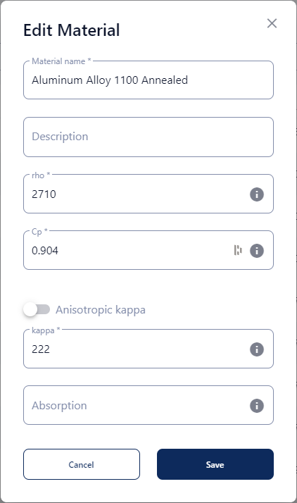
A constant value at a reference temperature: \(\kappa=100\)
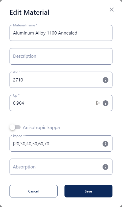
A polynomial in function of temperature where a maximum of 8 coefficients can be provided: \(\kappa=[1,2,3,4,5,6,7,8]\) This array represents the coefficients of a polynomial: \(\kappa = 1 + 2T + 3T^{2} + 4T^{3} + 5T^{4} + 6T^{5} + 7T^{6} + 8T^{7}\)
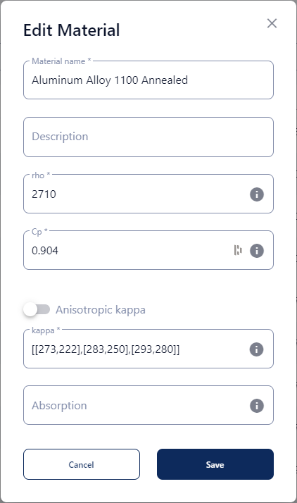
A table containing the temperature and corresponding parameter value of the material at the specified temperature: \(\kappa=[[273,100],[283,110],[293,120],[303,120]]\)